How Do I Show A Negative Percentage In Excel
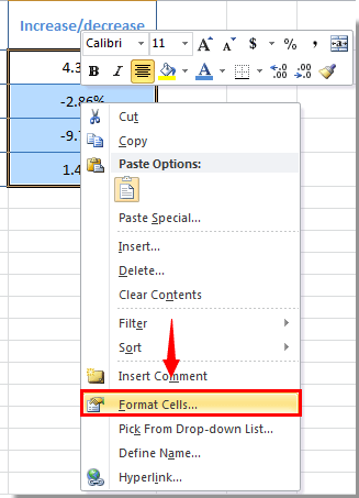
I have been able to format single cells to display negative percents Budget to Actual hours but I cannot copy the formatting to cells with positive percents without eliminating the format style I want. Hi Right click on the cell you want to format choos format cells choos the.

Displaying Negative Numbers In Parentheses Excel
Select the data range that you want to hide the negative numbers.
How do i show a negative percentage in excel. In this tutorial we will discover how to use the basic percentage formula calculate percentages in excel and explore different formulas for calculating percentage increase. Select the range of cells you want to format. Select the cell or cells that contain negative percentages.
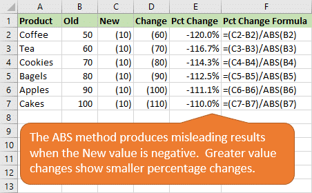
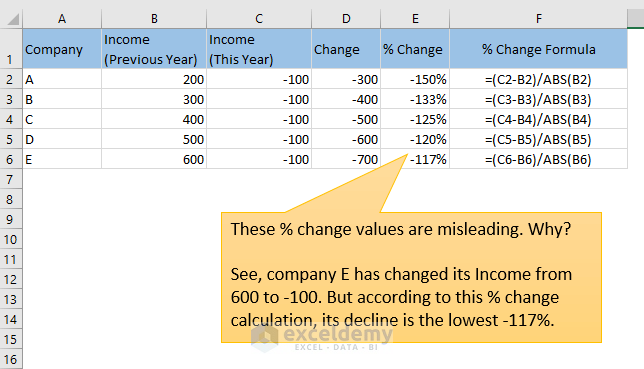
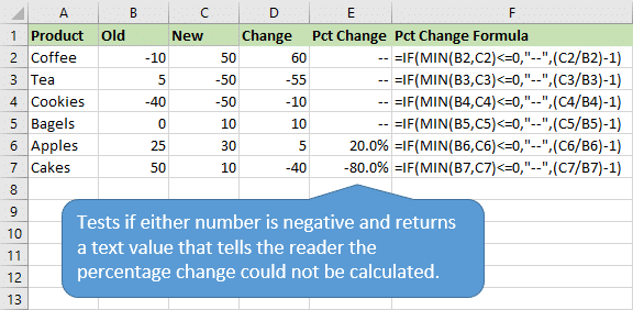
Heres how you do it. Add Brackets. C4-B4ABS B4 The figure uses this formula in cell E4 illustrating the different results you get when using the standard percent variance formula and the improved percent variance formula.
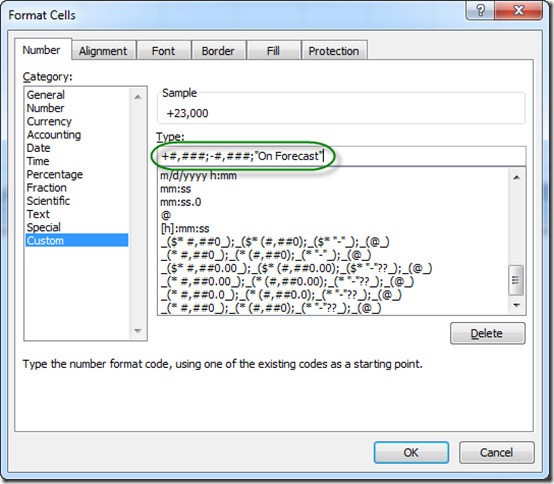
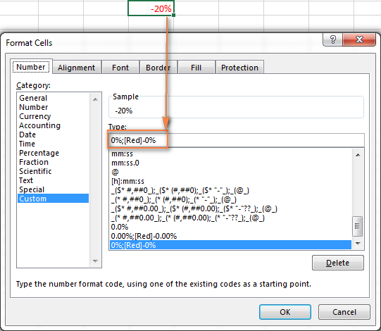
For the 8 decrease enter this excel percentage formula in b19. Number tab choos custom enter in the Type text box. In the Format Cells dialog box you need to.
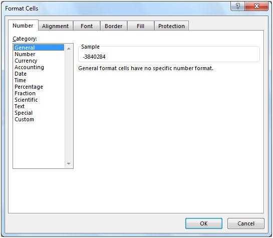
Excel formula for percentage change percentage increase decrease. On the Home tab click Format Format Cells. Blue 0 Each symbol has a meaning and in this format the represents the display of a significant digit and the 0 is the display of an insignificant digit.
Hide negative numbers in Excel with Conditional Formatting. In the Format Cells box in the Category list click Custom. What makes you think so.
To select multiple cells hold down the Ctrl key as you. When a formula returns a negative percentage the result is formatted as -49. This negative number is enclosed in parenthesis and also displayed in blue.
The Conditional Formatting may help you to hide the value if negative please do with the following steps. Or hit CTRL1 to open the format cells dialog box. Be sure to subscribe to the newsletter for more Excel tips and tricks.
A common way is to mark negative variances to budget in red and positive in black. Is there any format in Excel 2002 that allows for it to be formatted 49. This is a time-honored way of formatting numbers as the sayings in the red and black Friday demonstrate.
Click Custom in. A B 1 -6249 -5810 A1B1 10756 The change is moving from B to A. Select the cell or cells that may contain negative percentages.
Negative Percentage in Parenthesis instead of with - sign. If you used -10756 arbitrarily. Right click the selected cells and select Format Cells in the right-clicking menu.
On the home tab in the number group click the increase decimal button once. Add Brackets Minus Sign Mark Red All Negative PercentagesIn this Excel tutorial you ar. Learn how to calculate the percent change or difference between two.
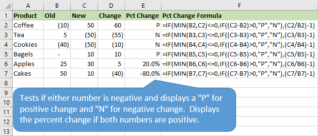
If I divide two negative numeric cells and put the result into a percentage cell it will positive even if the change is negative. How to Mark Negative Percentage in Red in Microsoft ExcelIn this Excel tutorial you are about to learn two distinctive ways to mark or display negative per. Percent Change Formula In Excel Easy Excel Tutorial.
000 hope this will work for you. In the Type box enter the following format. Percent Difference Formula Excel.
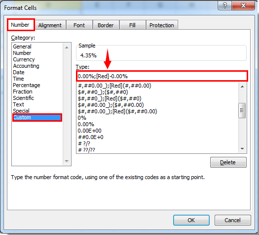
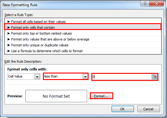
Click Home Conditional Formatting Highlight Cells Rules Less Than see screenshot. If you want to format negative percentages in a different way say in red font you can create a custom number format. I need to display with the parenthesis 136for negative results but say 186 for positive results.
This is just as easy to do at the same time as applying the postive conditional formatting. Add Parenthesis to Negative Percentages. Open the Format Cells dialog again navigate to the Number tab Custom category and enter one of the below formats in the Type box.
You can always use a custom format FormatCellsNumberCustom Type. That means I should have a negative change. Choose Conditional Formatting from the Format menu.
One common way to calculate percentage change with negative numbers it to make the denominator in the formula positive. Select the cells which have the negative percentage you want to mark in red. -581010756 is -6249 the correct answer.
In the Type box enter the code below. How to make all negative numbers in red in Excel. The other way that you can display negative percentages in red is to use conditional formatting by following these steps.
Red-000 - format negative percentages in red and display 2 decimal places. The fix is to leverage the ABS function to negate the negative benchmark value.
How To Make All Negative Numbers In Red In Excel
Display Plus Sign In Excel If Value Is Positive Blog
How To Make All Negative Numbers In Red In Excel
Calculate Percentage Change For Negative Numbers In Excel Excel Campus
Calculate Percentage Change For Negative Numbers In Excel Excel Campus
Calculate Percentage Change For Negative Numbers In Excel Excel Campus
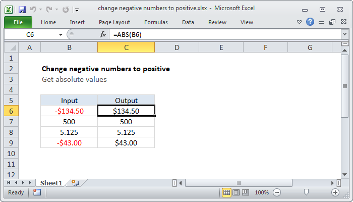
Excel Formula Change Negative Numbers To Positive Exceljet

7 Amazing Excel Custom Number Format Tricks You Must Know
How To Make All Negative Numbers In Red In Excel

Displaying Negative Numbers In Parentheses Excel
How To Show Percentage In Excel
Excel Formula Cap Percentage At 100 Exceljet
Excel Find Difference Between Two Numbers Positive Or Negative

How To Display Negative Percentages In Red Within Brackets In Excel Excel Tutorials Excel Negativity

How To Make All Negative Numbers In Red In Excel
Formatting A Negative Number With Parentheses In Microsoft Excel
Kb40241 The Negative Percentage Values In A Graph Report Are Displayed Outside The Parenthesis In Microstrategy Web And Developer 10 X

How To Show Percentage In Excel
Calculate Percentage Change For Negative Numbers In Excel Excel Campus